No matter the number of new pitching metrics invented by sabermetricians today, it seems increasingly more difficult to supplant WHIP as one of the (if not THE) premier pitching metrics.
Monthly Archives: April 2013
Performance vs. Production
Special thanks to Harry Pavlidis (@HarryPav) for supplying me with the HITf/x data (April ’09 public release) earlier tonight. As I’m new to the world of practicing sabermetrics, I appreciated his introductory article.
Growing up when at the plate, I was taught by my Dad and other coaches to “find a way to get it done.” If a bloop single scored the run, then I succeeded. It wasn’t until I became a coach myself that my perspective changed (slightly). I began coaching five years ago and was introduced to the concept “Performance vs. Production.” Defined below:
Performance – the execution of an action. In baseball, a hitter’s performance is the sum of all actions within his control. It’s how he performs.
Production – something produced; output. That is, a hitter’s production is the outcome of his performance. It’s what he produces.
I’ve appreciated the increasing desire for sabermetricians to understand a player’s value without external factors. Tailored statistics such as DIPS, FIP, and tERA have provided us with the ability to analyze pitchers without influence from the other 8 players on the field. Even without context such as the out/base state or Tango’s leverage index, these provide outstanding value.
The “Performance vs. Production” philosophy teaches us to focus on what we can control. A hitter who crushed a ball with a 100+ mph exit velocity at a +10 degree angle (from horizontal) may not get out of the box as the third baseman snares the line drive. In the old days, this scenario would have me believe that I did nothing but fail. However, I now realize how the 100+ mph hitter above actually performed at an extraordinarily high level, yet his production fell to some bad luck. When analyzing how a hitter performs, we must temporarily remove the outcome and focus on what the hitter can control. Fundamentally, three basic factors describe a hitter’s performance: the exit velocity off his bat, the launch angle, and the spray angle.
In developing this philosophy, I’ll make the sweeping assumption that a hitter cannot control his spray angle. (Yes, our eyes and spray charts tell us that certain players like Ortiz & Bonds predominantly pull the baseball.) However at the macro scale, most “good” hitters hit the ball where it’s pitched. That is, a hitter keeps his hands inside the baseball on an inside pitch to barrel it to his pull side while outside pitches are allowed to get deeper and are taken to the oppo field. On the micro level, hitters are taught to keep their bat through the hitting zone longer; once his hands have started and his bat travels through the zone, his bat spray angle continuously changes with no ability to make an adjustment without severely sacrificing bat speed.
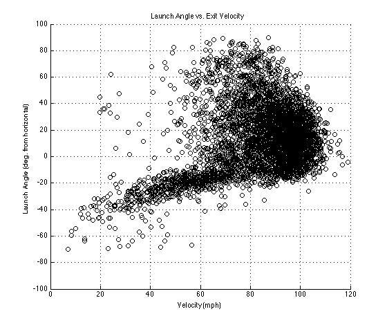
Therefore, we’ll focus on the two factors a hitter most certainly can control: ball exit velocity and launch angle. Traditionally these are recognized as “bat speed” and “timing,” respectively. A quick analysis of the available HITf/x data shows a distribution of each of these factors below.

Notice the average at bat produced a ball exit velocity of 82.3 mph at a launch angle 13.3 degrees above horizontal.

Now plotting every batted ball’s launch angle/exit velocity combination, we observe the following scatter plot.
This is where things get interesting (and fun). We can now view the two factors within a hitter’s control in one location. However, we need to find a way to measure it. Long term, increased performance will lead to increased production. So let’s measure the performance. Tango’s wOBA is awesome, however it focuses on a hitter’s production. A hitter can’t control how an opposing player fields his batted ball, so why should we measure his value based off of these factors? A hitter has virtually no control over reaching on errors, and I would argue (at the MLB level) he has very little control over HBPs. [I'm a long time HBP advocate for players as long as they are properly taught how to protect themselves (maybe a future teaching post). Yes, he controls where he stands in the box and how he reacts to an inside pitch, but in general, HBPs are controlled by the pitcher.] Even singles, doubles, and triples possess a large defensive bias.
Therefore, let’s remove luck, chance, and defensive alignment/skill and evaluate a hitter’s performance. To do so, we’ll take a look at what exit velocity and launch angle combinations will lead to expected outcomes. I’ve broken down the two factors into 40 “bins.” Specifically, I broke exit velocity into 4 mph increments and launch angle into 3 degree increments. Therefore, the 40×40 matrix provides 1,600 bins (many are empty, grey). Within each bin, a certain number of batted balls were tracked and marked with a specific outcome (e.g. out, single, HR, etc.) I then averaged the wOBA within each 4 mph x 3 degree bin. The heat map below displays the outcome of that analysis. Red & yellow denote high wOBA (HRs & XBH’s); teal/green depict medium wOBA (think singles); blue represents poor wOBA (outs). Optimal hitting occurs approximately between 18-40 degrees in excess of 95 mph.
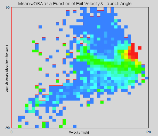
Due to the limited data set (< 5,000 AB’s), the resolution is grainy, at best. I’m imagining Sportvision’s database by now would provide quite an elegant heat map. Given the opportunity to analyze realtime HITf/x data, I would measure a hitter’s performance using Tango’s wOBA as a foundation. However, in lieu of assigning the linear weight associated with the outcome of a hitter’s AB, let’s analyze the exit velocity and launch angle, then use a LUT (look up table, with significantly higher resolution) to find the average linear weight associated with all balls hit within that bin. Accounting for all hits, outs, and ROEs then averaging will enable us to substantially reduce performance increase/suppression due to factors external to the hitter. This allows us to utilize the large data set of the broad population to analyze an individual hitter’s performance. Maybe we call it pOBA (Performance On-Base Average).
We could then make an adjustment for baserunning speed/ability using FIELDf/x. For balls hit to the outfield, we could then easily perform park adjustments, if desired. After all, in the infield, home to 1st is 88′ – 9″ regardless of the stadium in which one plays. Pair our newly created context independent pOBA statistic with my longtime favorite RE24, and you’ve got an incredible analysis for MLB hitters.
Game Theory: Down Angle
Let’s talk managerial strategy. Imagine runners on 2nd & 3rd with 1 out and the defense is “playing in.” As a baserunner at 3rd, how are you instructed to react on a groundball? Most likely, you’re taught to “see it through the infield.” But should you? Let’s evaluate the decision using some numbers.
Before we begin, we need to understand a concept called “run expectancy” (RE). Given any base/out situation, the RE is the average number of runs scored from that moment until the end of that inning. This can be found empirically (off historical data) or through simulations (using Markov chains). Tom Tango founded this idea using MLB data more than a decade ago. We’ve followed his lead using the empirical approach with NCAA data since the adoption of BBCOR bat restrictions.
Back to our situation: 2nd & 3rd with 1 out. The NCAA RE in this situation is 1.562 runs, but that’s not so important. What we want to evaluate is the RE after this play is complete. Depending on the baserunning decision our final RE may be different. To keep the complexity of this evaluation to a minimum, we need to establish a few assumptions.
Assumption 1. Only one error may be made on a play, and any error made does not advance baserunners any further than the base they already exist. (Think throwing error caught by 1B that pulls him off the bag.)
Assumption 2. The 3rd base coach has clairvoyance in deciding the fate of the runner at 2nd (and 2nd only). In other words, on a single, he’s always perfect in his decision on whether or not to send the runner home when rounding 3rd. If he’ll be out, he holds him at 3rd. If he’ll score, he waves him home.
Assumption 3. The hitter will never end up past further than 1st base. Clearly there are several scenarios in which this could occur, however to eliminate complexity, we’ll stick with this as our final assumption.
Now we can move to our decision. As described earlier, we have two options. First, we have the traditional “see it through the infield” choice. Second, we have our “down angle” philosophy. Each decision has it’s related outcomes.
Option 1. Runners freeze until the ball is through the infield, then advance. Given a routine groundball, this option has four basic possible outcomes A – D.
A – Hitter grounds out. Runners remain at 2nd & 3rd. 0 runs scored. 2 outs.
B – Hitter grounds to a fielder who makes an error. Runners remain at 2nd & 3rd, and the hitter is safe at 1st. 0 runs scored. 1 out.
C – Hitter singles through the infield. Because they froze to see the ball through, runners move up one base each. Hitter is safe at 1st. Baserunners now at 1st & 3rd. 1 run scored. 1 out.
D – Hitter singles through the infield. Although they froze, both runners ended up scoring. Hitter is safe at 1st. 2 runs scored. 1 out.
Option 2. Runners move on down angle contact. That is, they advance upon a downward launch angle regardless of the spray angle. Given a routine groundball, this option has five potential outcomes E – J.
E – Hitter grounds into a FC as a fielder throws home to tag the runner out. Runners now at 1st & 3rd. 0 runs scored. 2 outs.
F – Hitter grounds to a fielder who makes an error. Runners now at 1st & 3rd. 1 run scored. 1 out.
G – Hitter singles through the infield. Although they were moving on contact, only one runner scored. Hitter is safe at 1st. Baserunners now at 1st & 3rd. 1 run scored. 1 out.
H – Hitter singles through the infield. Because they were moving on contact, both runners were able to score. Hitter is safe at 1st. 2 runs scored. 1 out.
J – Hitter grounds to a fielder who is unable to make the play at home, but can make the play at 1st. Runner from 2nd advances to 3rd. 1 run scored. 2 outs.
Assigning Probabilities:
Now that we’ve identified the two options and their corresponding potential outcomes, it’s time to apply some probabilities of occurrence for each specific outcome. Then, we can complete the decisional analysis. Our justification:
1. The average NCAA fielding percentages on all plays is 0.965 (thus, the error in decision #1 has a 3.5% chance of occurring). However, the play at home is unique and rare. Therefore, we’ll assume that an error here occurs twice as often, so a 7.0% chance of occurrence. (Runner has a lead, is off on contact, and it’s a tag play at home. Many more variables than a standard 6-3 putout.)
2. Given the ball is hit on the ground with the infield in, the ball will get through for a single 40% (estimated) of the time.
3. Of all singles with 1 out, a runner on 2nd will score on 47.6% of them when a runner reacts normally (doesn’t freeze to see the ball through the infield). When freezing, the runner on 2nd will score approximately 25% of the time.
4. 10% of the groundballs will result in a fielder being unable to make a play at home, but will be able to get the out at 1st (think diving stop, but not enough time to throw home).
Analyzing the traditional “see it through the infield” decision:
| Decision | Outcome | Bases Occupied | Runs Scored | Outs Remaining | RE of End State | Runs + RE | Probability of Occurance | e-Value |
| 1 | A | _23 | 0 | 2 | 0.684 | 0.684 | 0.665 | 0.45 |
| 1 | B | 123 | 0 | 1 | 1.792 | 1.792 | 0.035 | 0.06 |
| 1 | C | 1_3 | 1 | 1 | 1.357 | 2.357 | 0.300 | 0.71 |
| 1 | D | 1__ | 2 | 1 | 0.630 | 2.630 | 0.100 | 0.26 |
| 1.49 |
And now the “down angle” method:
| Decision | Outcome | Bases Occupied | Runs Scored | Outs Remaining | RE of End State | Runs + RE | Probability of Occurance | e-Value |
| 2 | E | 1_3 | 0 | 2 | 0.611 | 0.611 | 0.430 | 0.26 |
| 2 | F | 1_3 | 1 | 1 | 1.357 | 2.357 | 0.070 | 0.16 |
| 2 | G | 1_3 | 1 | 1 | 1.357 | 2.357 | 0.210 | 0.49 |
| 2 | H | 1__ | 2 | 1 | 0.630 | 2.630 | 0.190 | 0.50 |
| 2 | J | __3 | 1 | 2 | 0.449 | 1.449 | 0.100 | 0.14 |
| 1.57 |
With the runs, outs, RE’s, and probabilities identified, we can compute an expected value, simply (Runs + RE) * probability. Without getting too technical, the final e-value is our new RE the moment the ball leaves the hitter’s bat on a negative launch angle. As we find a value for each decision, we want to continually choose the higher (assuming risk neutrality) to generate more runs over time. Thus, long term, the down angle philosophy will increase RE by 0.08 runs. Next week, we’ll provide a sensitivity analysis to determine how dependent our findings are to the various assigned probabilities.
Remember, you can’t evaluate a decision based on it’s outcome. Separate the two. In summary, go down angle… and go home.
RBI Hitting Approach: Should it Change?
Having had a lengthy discussion with the three other coaches on our collegiate staff regarding a hitter’s approach with RISP, I thought I’d make an attempt to analyze how professional hitters might alter their approach in RBI situations. Specifically, we’re focusing on runners at 3rd or 2nd/3rd with less than 2 outs. We have eliminated all situations in which a runner resides on 1st since a coach/manager may elect to employ a strategic play (e.g. a hit & run). We have also eliminated all bunt attempts from this study. We truly want to evaluate the approach a hitter may take without external factors such as managerial strategy.
With a proven, established approach already in place in our college program, a new perspective provided the suggestion to be more aggressive and “eat the RBI early.” That is, a hitter in an RBI situation ought to look for something he can hit early in the count. This philosophy to “look for something you can hit versus drive” may allow one to avoid more strikeouts, but will it lead to success?
First, let’s establish the “standard” approach. Seems to me, the simplest situation is 0 on, 0 out. A hitter’s goal is to simply get on base. With 500,011 MLB PA’s from 2002-2012, this is clearly enough data to establish our standard. (Other situations such as 0 on, 1 out could be considered, however certain nuances of the game could affect the P/PA. For example, a 1-pitch AB by the leadoff hitter may force the second hitter of the inning to take a pitch to avoid the quick inning.) Nevertheless, we find 3.8175 P/PA with 0 on and 0 outs.
Baserunning 101: Home to 1st is not 90′
Again, home to 1st is not 90′.
It’s 88′-9″.

When baseball was created, the 90 feet we all know was defined as the distance to the baselines. However, 1st (and 3rd) base are situated on/inside the 90 degree angle that the baselines create. Now, you may be asking yourself, “who cares?” In reality, nobody should really care about the actual distance from home to 1st (it really is 88′-9″ from the back corner of home plate to the FRONT of 1st base… 90′ baseline minus a 15″ base).
The key here, is the word “front.” When telling yourself, or teaching another, to run to first base, encourage him/her to hit the front part of the bag. How so? Well this is something that can’t quite be explicitly taught. Even sabermetrics won’t help us here (yet). What you can do, however, is get out of the box and run hard. Then, with three strides remaining, make a small adjustment to slightly lengthen or shorten your strides to ensure you hit the front (not middle, not back) part of the bag. This adjustment requires athleticism and that “feel” for the game we all look for.
Too many times (from little league to the pros), we’ve witnessed players hit the back half of the base rather than the front. Sometimes, even, they won’t hit it at all.
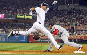
Picture courtesy of the NY Times
Focus on the little things to improve your game.
The Creation of ePPA: Estimating P/PA Given Count Information
With the wealth of information available at the MLB level, P/PA (pitches per plate appearance) data can be easily queried through your favorite database. (I currently use a combination of MySQL, MATLAB, and R for all of our analytics here at Diamond Charts.) However, at the collegiate level, detailed P/PA data must be derived from the pitch count. Sounds simple, but don’t forget that two-strike foul balls aren’t accounted for in a standard play-by-play. Therefore, in order to provide a slightly more accurate P/PA estimation, we’ve created ePPA (estimated P/PA) to account for those foul balls that occur with two strikes. Methodology is below.
Assumption: NCAA hitters foul off as many 2-strike pitches as MLB hitters. (Later we can turn this assumption into a hypothesis and test its validity.)
Utilizing MLB PBP data from 2002-2012, we find 1.003M PA’s with two strikes prior to the action pitch. During these PA’s we find an actual P/PA of 5.11 while observing a count-based P/PA (simply, balls + strikes + 1) of 4.62. The plot below displays the distribution of total strikes encompassing all 1.003M 2-strike MLB PA’s over the past decade. As we can see, approximately 70% of PA’s with 2 strikes have 2 total strikes (that is, they have 0 fouls on 2 strike counts). However an adjustment clearly remains necessary for the other 30%. In case you’re curious, the most number of total strikes seen in one PA in the past decade occurred in 2004 in Los Angeles as Alex Cora of the Dodgers homered off Matt Clement of the Chicago Cubs in an 18 pitch at-bat.

One step further:
In order to more accurately find an ePPA that approximates more closely to the actual P/PA, we have broken these numbers down into the four possible 2-strike counts. The table below displays the actual P/PA with the count based P/PA (cPPA = balls + strikes + 1) and the difference between them.
| balls_ct | P/PA | cPPA | diff |
| 0 | 3.243 | 3 | 0.243 |
| 1 | 4.370 | 4 | 0.370 |
| 2 | 5.533 | 5 | 0.533 |
| 3 | 6.747 | 6 | 0.747 |
The chart makes sense, the more balls/pitches a hitter sees, the more opportunities he has to foul off a 2-strike pitch. Thus, for every 2-strike PA, we add the differential factor based upon the number of balls in the count, providing a slightly more accurate representation of ePPA (ePPA = cPPA + diff). Because P/PA is a cumulative statistic (one that should be analyzed over a large data set), these simplistic approximations will suffice.
Effect:
2-strike counts make up approximately half of all plate appearances, thus providing an overall addition of approximately 0.24 P/PA for each hitter (a bit more for more patient hitters, a bit less for the aggressive). Thinking differently, on the order of 10 foul balls/game (per team) occur with two strikes.
Hello to the Sabermetric Community
Hello to all baseball fans, coaches, players, front office personnel, and sabermetricians. Having launched Diamond Charts just a few months ago, we are at the infant stages of our dive into the sabermetric world. We’ve created this sabrlog as a fun outlet to document our endeavor. We encourage discussion and hope you won’t hesitate to point out flaws, whether in methodology or even simple oversights.
As former collegiate players and a current coach, we enjoy teaching the game. Thus, this sabrlog may also include a sprinkling of (hopefully) interesting aspects related to the fundamentals of baseball. Our current focus is on the collegiate game, so many of our articles will focus on some aspect of it. However we’ll often use MLB data to “learn from the pros” and make inferences to improve the college game. We’ll strive to provide high quality articles (in lieu of high quantity) that are both on point, yet deep enough to provide an accurate analysis. We hope you enjoy.
All the best,
Diamond Charts
[Twitter @DiamondCharts]